Survival Analysis for Deep Learning
Most machine learning algorithms have been developed to perform classification or regression. However, in clinical research we often want to estimate the time to and event, such as death or recurrence of cancer, which leads to a special type of learning task that is distinct from classification and regression. This task is termed survival analysis, but is also referred to as time-to-event analysis or reliability analysis. Many machine learning algorithms have been adopted to perform survival analysis: Support Vector Machines, Random Forest, or Boosting. It has only been recently that survival analysis entered the era of deep learning, which is the focus of this post.
You will learn how to train a convolutional neural network to predict time to a (generated) event from MNIST images, using a loss function specific to survival analysis. The first part , will cover some basic terms and quantities used in survival analysis (feel free to skip this part if you are already familiar). In the second part , we will generate synthetic survival data from MNIST images and visualize it. In the third part , we will briefly revisit the most popular survival model of them all and learn how it can be used as a loss function for training a neural network. Finally , we put all the pieces together and train a convolutional neural network on MNIST and predict survival functions on the test data.
The notebook to reproduce the results is available on GitHub, or you can run it directly using Google Colaboratory.
Primer on Survival Analysis
The objective in survival analysis is to establish a connection between covariates and the time of an event. The name survival analysis originates from clinical research, where predicting the time to death, i.e., survival, is often the main objective. Survival analysis is a type of regression problem (one wants to predict a continuous value), but with a twist. It differs from traditional regression by the fact that parts of the training data can only be partially observed – they are censored.
As an example, consider a clinical study that has been carried out over a 1 year period as in the figure below.

Patient A was lost to follow-up after three months with no recorded event, patient B experienced an event four and a half months after enrollment, patient C withdrew from the study two months after enrollment, and patient E did not experience any event before the study ended. Consequently, the exact time of an event could only be recorded for patients B and D; their records are uncensored. For the remaining patients it is unknown whether they did or did not experience an event after termination of the study. The only valid information that is available for patients A, C, and E is that they were event-free up to their last follow-up. Therefore, their records are censored.
Formally, each patient record consists of the time $t>0$ when an event occurred or the time $c>0$ of censoring. Since censoring and experiencing an event are mutually exclusive, it is common to define an event indicator $\delta \in \{0;1\}$ and the observable survival time $y>0$. The observable time $y$ of a right censored time of event is defined as
$$ y = \min(t, c) = \begin{cases} t & \text{if } \delta = 1 , \\% c & \text{if } \delta = 0 . \end{cases} $$
Consequently, survival analysis demands for models that take partially observed, i.e., censored, event times into account.
Basic Quantities
Typically, the survival time is modelled as a continuous non-negative random variable $T$, from which basic quantities for time-to-event analysis can be derived, most importantly, the survival function and the hazard function.
- The survival function $S(t)$ returns the probability of survival beyond time $t$ and is defined as $S(t) = P(T > t)$. It is non-increasing with $S(0) = 1$, and $S(\infty) = 0$.
- The hazard function $h(t)$ denotes an approximate probability (it is not bounded from above) that an event occurs in the small time interval $[t; t + \Delta[$, under the condition that an individual would remain event-free up to time $t$: $$ h(t) = \lim_{\Delta t \rightarrow 0} \frac{P(t \leq T < t + \Delta t \mid T \geq t)}{\Delta t} \geq 0 $$ Alternative names for the hazard function are conditional failure rate, conditional mortality rate, or instantaneous failure rate. In contrast to the survival function, which describes the absence of an event, the hazard function provides information about the occurrence of an event.
Generating Synthetic Survival Data from MNIST
To start off, we are using images from the MNIST dataset and will synthetically generate survival times based on the digit each image represents. We associate a survival time (or risk score) with each class of the ten digits in MNIST. First, we randomly assign each class label to one of four overall risk groups, such that some digits will correspond to better and others to worse survival. Next, we generate risk scores that indicate how big the risk of experiencing an event is, relative to each other.
| risk_score | risk_group | |
|---|---|---|
| class_label | ||
| 0 | 3.071 | 3 |
| 1 | 2.555 | 2 |
| 2 | 0.058 | 0 |
| 3 | 1.790 | 1 |
| 4 | 2.515 | 2 |
| 5 | 3.031 | 3 |
| 6 | 1.750 | 1 |
| 7 | 2.475 | 2 |
| 8 | 0.018 | 0 |
| 9 | 2.435 | 2 |
We can see that class labels 2 and 8 belong to risk group 0, which has the lowest risk (close to zero). Risk group 1 corresponds to a risk score of about 1.7, risk group 2 of about 2.5, and risk group 3 is the group with the highest risk score of about 3.
To generate survival times from risk scores, we are going to follow the protocol of Bender et al. We choose the exponential distribution for the survival time. Its probability density function is $f(t\,|\,\lambda) = \lambda \exp(-\lambda t)$, where $\lambda > 0$ is a scale parameter that is the inverse of the expectation: $E(T) = \frac{1}{\lambda}$. The exponential distribution results in a relatively simple time-to-event model with no memory, because the hazard rate is constant: $h(t) = \lambda$. For more complex cases, refer to the paper by Bender et al.
Here, we choose $\lambda$ such that the mean survival time is 365 days. Finally, we randomly censor survival times drawing times of censoring from a uniform distribution such that we approximately obtain the desired amount of 45% censoring. The generated survival data comprises an observed time and a boolean event indicator for each MNIST image.
We can use the generated censored data and estimate the survival function $S(t)$ to see what the risk scores actually mean in terms of survival. We stratify the training data by class label, and estimate the corresponding survival function using the non-parametric Kaplan-Meier estimator.

Classes 0 and 5 (dotted lines) correspond to risk group 3, which has the highest risk score. The corresponding survival functions drop most quickly, which is exactly what we wanted. On the other end of the spectrum are classes 2 and 8 (solid lines) belonging to risk group 0 with the lowest risk.
Evaluating Predictions
One important aspect for survival analysis is that both the training data and the test data are subject to censoring, because we are unable to observe the exact time of an event no matter how the data was split. Therefore, performance measures need to account for censoring. The most widely used performance measure is Harrell’s concordance index. Given a set of (predicted) risk scores and observed times, it checks whether the ordering by risk scores is concordant with the ordering by actual survival time. While Harrell’s concordance index is widely used, it has its flaws, in particular when data is highly censored. Please refer to my previous post on evaluating survival models for more details.
We can take the risk score from which we generated survival times to check how good a model would perform if we knew the actual risk score.
cindex = concordance_index_censored(event_test, time_test, risk_scores[y_train.shape[0]:])

print(f"Concordance index on test data with actual risk scores: {cindex[0]:.3f}")
Concordance index on test data with actual risk scores: 0.705
Surprisingly, we do not obtain a perfect result of 1.0. The reason for this is that generated survival times are randomly distributed based on risk scores and not deterministic functions of the risk score. Therefore, any model we will train on this data should not be able to exceed this performance value.
Cox’s Proportional Hazards Model
By far the most widely used model to learn from censored survival data, is Cox’s proportional hazards model model. It models the hazard function $h(t_i)$ of the $i$-th subject, conditional on the feature vector $\mathbf{x}_i \in \mathbb{R}^p$, as the product of an unspecified baseline hazard function $h_0$ (more on that later) and an exponential function of the linear model $\mathbf{x}_i^\top \mathbf{\beta}$:
$$ h(t | x_{i1}, \ldots, x_{ip}) = h_0(t) \exp \left( \sum_{j=1}^p x_{ij} \beta_j \right) \Leftrightarrow \log \frac{h(t | \mathbf{x}_i)}{h_0 (t)} = \mathbf{x}_i^\top \mathbf{\beta} , $$
where $\mathbf{\beta} \in \mathbb{R}^p$ are the coefficients associated with each of the $p$ features, and no intercept term is included in the model. The key is that the hazard function is split into two parts: the baseline hazard function $h_0$ only depends on the time $t$, whereas the exponential is independent of time and only depends on the covariates $\mathbf{x}_i$.
Cox’s proportional hazards model is fitted by maximizing the partial likelihood function, which is based on the probability that the $i$-th individual experiences an event at time $t_i$, given that there is one event at time point $t_i$. As we will see, by specifying the hazard function as above, the baseline hazard function $h_0$ can be eliminated and does not need be defined for finding the coefficients $\mathbf{\beta}$. Let $\mathcal{R}_i = \{ j\,|\,y_j \geq y_i \}$ be the risk set, i.e., the set of subjects who remained event-free shortly before time point $y_i$, and $I(\cdot)$ the indicator function, then we have
$$ \begin{aligned} &P(\text{subject experiences event at $y_i$} \mid \text{one event at $y_i$}) \\% =& \frac{P(\text{subject experiences event at $y_i$} \mid \text{event-free up to $y_i$})} {P (\text{one event at $y_i$} \mid \text{event-free up to $y_i$})} \\% =& \frac{h(y_i | \mathbf{x}_i)}{ \sum_{j=1}^n I(y_j \geq y_i) h(y_j | \mathbf{x}_j) } \\% =& \frac{h_0(y_i) \exp(\mathbf{x}_i^\top \mathbf{\beta})} { \sum_{j=1}^n I(y_j \geq y_i) h_0(y_j) \exp(\mathbf{x}_j^\top \mathbf{\beta}) } \\% =& \frac{\exp( \mathbf{x}_i^\top \beta)}{\sum_{j \in \mathcal{R}_i} \exp( \mathbf{x}_j^\top \beta)} . \end{aligned} $$
By multiplying the conditional probability from above for all patients who experienced an event, and taking the logarithm, we obtain the partial likelihood function:
$$ \widehat{\mathbf{\beta}} = \arg\max_{\mathbf{\beta}}~ \log\,PL(\mathbf{\beta}) = \sum_{i=1}^n \delta_i \left[ \mathbf{x}_i^\top \mathbf{\beta} - \log \left( \sum_{j \in \mathcal{R}_i} \exp( \mathbf{x}_j^\top \mathbf{\beta}) \right) \right] . $$
Non-linear Survival Analysis with Neural Networks
Cox’s proportional hazards model as described above is a linear model, i.e., the predicted risk score is a linear combination of features. However, the model can easily be extended to the non-linear case by just replacing the linear predictor with the output of a neural network with parameters $\mathbf{\Theta}$.

This has been realized early on and was originally proposed in the work of Faraggi and Simon back in 1995. Farragi and Simon explore multilayer perceptrons, but the same loss can be used in combination with more advanced architectures such as convolutional neural networks or recurrent neural networks. Therefore, it is natural to also use the same loss function in the era of deep learning. However, this transition is not so easy as it may seem and comes with some caveats, both for training and for evaluation.
Computing the Loss Function
When implementing the Cox PH loss function, the problematic part is the inner sum over the risk set: $\sum_{j \in \mathcal{R}_i} \exp( \mathbf{x}_j^\top \mathbf{\beta})$. Note that the risk set is defined as $\mathcal{R}_i = \{ j\,|\,y_j \geq y_i \}$, which implies an ordering according to observed times $y_i$, which may lead to quadratic complexity if implemented naively. Ideally, we want to sort the data once in descending order by survival time and then incrementally update the inner sum, which leads to a linear complexity to compute the loss (ignoring the time for sorting).
Another problem is that the risk set for the subject with the smallest uncensored survival time is over the whole dataset. This is usually impractical, because we may not be able to keep the whole dataset in GPU memory. If we use mini-batches instead, as it’s the norm, (i) we cannot compute the exact loss, because we may not have access to all samples in the risk set, and (ii) we need to sort each mini-batch by observed time, instead of sorting the whole data once.
For practical purposes, computing the Cox PH loss over a mini-batch is usually fine, as long as the batch contains several uncensored samples, because otherwise the outer sum in the partial likelihood function would be over an empty set. Here, we implement the sum over the risk set by multiplying the exponential of the predictions (as a row vector) by a squared boolean matrix that contains each sample’s risk set as its rows. The sum over the risk set for each sample is then equivalent to a row-wise summation.
class InputFunction:
    …

    def _get_data_batch(self, index):
        """Compute risk set for samples in batch."""
        time = self.time[index]
        event = self.event[index]
        images = self.images[index]

        labels = {
            "label_event": event.astype(np.int32),
            "label_time": time.astype(np.float32),
            "label_riskset": _make_riskset(time)
        }
        return images, labels
    …

def _make_riskset(time):
    assert time.ndim == 1, "expected 1D array"

    # sort in descending order
    o = np.argsort(-time, kind="mergesort")
    n_samples = len(time)
    risk_set = np.zeros((n_samples, n_samples), dtype=np.bool_)
    for i_org, i_sort in enumerate(o):
        ti = time[i_sort]
        k = i_org
        while k < n_samples and ti == time[o[k]]:
            k += 1
        risk_set[i_sort, o[:k]] = True
    return risk_set

def coxph_loss(event, riskset, predictions):
    # move batch dimension to the end so predictions get broadcast
    # row-wise when multiplying by riskset
    pred_t = tf.transpose(predictions)
    # compute log of sum over risk set for each row
    rr = logsumexp_masked(pred_t, riskset, axis=1, keepdims=True)

    losses = tf.multiply(event, rr - predictions)
    loss = tf.reduce_mean(losses)
    return loss

def logsumexp_masked(risk_scores, mask,
                     axis=0, keepdims=None):
    """Compute logsumexp across `axis` for entries where `mask` is true."""
    mask_f = tf.cast(mask, risk_scores.dtype)
    risk_scores_masked = tf.multiply(risk_scores, mask_f)
    # for numerical stability, substract the maximum value
    # before taking the exponential
    amax = tf.reduce_max(risk_scores_masked, axis=axis, keepdims=True)
    risk_scores_shift = risk_scores_masked - amax

    exp_masked = tf.multiply(tf.exp(risk_scores_shift), mask_f)
    exp_sum = tf.reduce_sum(exp_masked, axis=axis, keepdims=True)
    output = amax + tf.log(exp_sum)
    if not keepdims:
        output = tf.squeeze(output, axis=axis)
    return output
To monitor the training process, we would like to compute the concordance index with respect to a separate validation set. Similar to the Cox PH loss, the concordance index needs access to predicted risk scores and ground truth of all samples in the validation data. While we had to opt for computing the Cox PH loss over a mini-batch, I would not recommend this for the validation data. For small batch sizes and/or high amount of censoring, the estimated concordance index would be quite volatile, which makes it very hard to interpret. In addition, the validation data is usually considerably smaller than the training data, therefore we can collect predictions for the whole validation data and compute the concordance index accurately.
Creating a Convolutional Neural Network for Survival Analysis on MNIST
Finally, after many considerations, we can create a convolutional neural network (CNN) to learn a high-level representation from MNIST digits such that we can estimate each image’s survival function. The CNN follows the LeNet architecture where the last linear has one output unit that corresponds to the predicted risk score. The predicted risk score, together with the binary event indicator and risk set, are the input to the Cox PH loss.
def model_fn(features, labels, mode, params):
    model = tf.keras.Sequential([
        tf.keras.layers.Conv2D(6, kernel_size=(5, 5), activation='relu', name='conv_1'),
        tf.keras.layers.MaxPooling2D(pool_size=(2, 2)),
        tf.keras.layers.Conv2D(16, (5, 5), activation='relu', name='conv_2'),
        tf.keras.layers.MaxPooling2D(pool_size=(2, 2)),
        tf.keras.layers.Flatten(),
        tf.keras.layers.Dense(120, activation='relu', name='dense_1'),
        tf.keras.layers.Dense(84, activation='relu', name='dense_2'),
        tf.keras.layers.Dense(1, activation='linear', name='dense_3')
    ])

    risk_score = model(features, training=is_training)

    if mode == tf.estimator.ModeKeys.TRAIN:
        loss = coxph_loss(
            event=tf.expand_dims(labels["label_event"], axis=1),
            riskset=labels["label_riskset"],
            predictions=risk_score)
        optim = tf.train.AdamOptimizer(learning_rate=params["learning_rate"])
        gs = tf.train.get_or_create_global_step()
        train_op = tf.contrib.layers.optimize_loss(loss, gs,
                                                learning_rate=None,
                                                optimizer=optim)
    else:
        loss = None
        train_op = None

    return tf.estimator.EstimatorSpec(
        mode=mode,
        loss=loss,
        train_op=train_op,
        predictions={"risk_score": risk_score})


train_spec = tf.estimator.TrainSpec(
    InputFunction(x_train, time_train, event_train,
                  num_epochs=15, drop_last=True, shuffle=True))

eval_spec = tf.estimator.EvalSpec(
    InputFunction(x_test, time_test, event_test))

params = {"learning_rate": 0.0001, "model_dir": "ckpts-mnist-cnn"}

estimator = tf.estimator.Estimator(model_fn, model_dir=params["model_dir"], params=params)
tf.estimator.train_and_evaluate(estimator, train_spec, eval_spec)
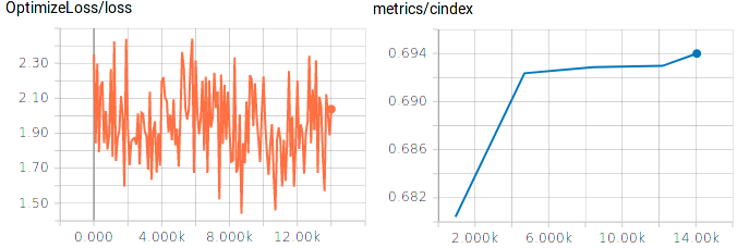
TensorBoard plots of training loss and concordance index on test data.
We can make a couple of observations:
- The final concordance index on the validation data is close to the optimal value we computed above using the actual underlying risk scores.
- The loss during training is quite volatile, which stems from the small batch size (64) and the varying number of uncensored samples that contribute to the loss in each batch. Increasing the batch size should yield smoother loss curves.
Predicting Survival Functions
For inference, things are much easier, we just pass a batch of images and record the predicted risk score. To estimate individual survival functions, we need to estimate the baseline hazard function $h_0$, which can be done analogous to the linear Cox PH model by using Breslow’s estimator.
from sklearn.model_selection import train_test_split
from sksurv.linear_model.coxph import BreslowEstimator


def make_pred_fn(images, batch_size=64):
    if images.ndim == 3:
        images = images[..., np.newaxis]

    def _input_fn():
        ds = tf.data.Dataset.from_tensor_slices(images)
        ds = ds.batch(batch_size)
        next_x = ds.make_one_shot_iterator().get_next()
        return next_x, None
    return _input_fn


train_pred_fn = make_pred_fn(x_train)
train_predictions = np.array([float(pred["risk_score"])
                              for pred in estimator.predict(train_pred_fn)])

breslow = BreslowEstimator().fit(train_predictions, event_train, time_train)
Once fitted, we can use Breslow’s estimator to obtain estimated survival functions for images in the test data. We randomly draw three sample images for each digit and plot their predicted survival function.
sample = train_test_split(x_test, y_test, event_test, time_test,
                          test_size=30, stratify=y_test, random_state=89)
x_sample, y_sample, event_sample, time_sample = sample[1::2]

sample_pred_fn = make_pred_fn(x_sample)
sample_predictions = np.array([float(pred["risk_score"])
                               for pred in estimator.predict(sample_pred_fn)])

sample_surv_fn = breslow.get_survival_function(sample_predictions)

Solid lines correspond to images that belong to risk group 0 (with lowest risk), which the model was able to learn. Samples from the group with the highest risk are shown as dotted lines. Their predicted survival functions have the steepest descent, confirming that the model correctly identified different risk groups from images.
Conclusion
We successfully built, trained, and evaluated a convolutional neural network for survival analysis on MNIST. While MNIST is obviously not a clinical dataset, the exact same approach can be used for clinical data. For instance, Mobadersany et al. used the same approach to predict overall survival of patients diagnosed with brain tumors from microscopic images, and Zhu et al. applied CNNs to predict survival of lung cancer patients from pathological images.
Sebastian Pölsterl
AI Researcher
My research interests include machine learning for time-to-event analysis, causal inference and biomedical applications.