Convolutional Autoencoder as TensorFlow estimator

In my previous post, I explained how to implement autoencoders as TensorFlow Estimator. I thought it would be nice to add convolutional autoencoders in addition to the existing fully-connected autoencoder. So that’s what I did. Moreover, I added the option to extract the low-dimensional encoding of the encoder and visualize it in TensorBoard.

The complete source code is available at https://github.com/sebp/tf_autoencoder.

Why convolutions?

For the fully-connected autoencoder, we reshaped each 28x28 image to a 784-dimensional feature vector. Next, we assigned a separate weight to each edge connecting one of 784 pixels to one of 128 neurons of the first hidden layer, which amounts to 100,352 weights (excluding biases) that need to be learned during training. For the last layer of the decoder, we need another 100,352 weights to reconstruct the full-size image. Considering that the whole autoencoder consists of 222,384 weights, it is obvious that these two layers dominate other layers by a large margin. When using higher resolution images, this imbalance becomes even more dramatic.

Convolutional layers allow us to significantly reduce the number of weights by sharing weights across multiple edges connecting pixels in the input image to the first hidden layer. A convolutional layer takes a small matrix of weights, let’s say 3x3, and slides it across the whole image as shown in the animation below (courtesy of Vincent Dumoulin and Francesco Visin):

The blue tiles represent the pixels of the input image, and the green tiles represent the output of the convolutional layer after multiplying each 3x3 patch in the input image with the 3x3 weight matrix and summing the result. This operation is called a convolution. To obtain an output – called feature map – of the same size as the input, we need to add a margin of 1 pixel (white tiles). Typical implementations of convolutions use the value of the closest true pixel for padded pixels. Having just a single 3x3 weight matrix in each layer is quite restrictive, thus we apply multiple convolutions on the same input, each with it’s own weight matrix. The big advantage is that the number of weights does not depend on the size of the input image, as it was the case for fully-connected layers, instead it is determined by the number of filters/kernels and their respective size (3x3 in the example above).

In the case of MNIST, inputs are $28 \times 28 \times 1$ gray-scale images with a single color channel, and the output of the first convolutional layer has as many “color” channels (feature maps) as there are filters, for example 16. The second convolutional layer will perform the same operation as the first layer, but on an “image” (or tensor to be more precise) of $28 \times 28 \times 16$.

Encoder

In the fully-connected autoencoder, we used layers with decreasing complexity by gradually decreasing the number of hidden units. When using convolutional layers in the encoder, we can reduce the complexity by lowering the number of filters or the resolution of the output. Two common approaches exist for down-scaling: 1) pooling values in a small window, 2) using convolutions with strides. The former introduces no additional weights, we simply compute the maximum/minimum/average over a small window – typically 2x2, which reduces width and height by a factor of 2. Note that the pooling operation is applied to each channel independently, thus the number of channels is not altered. Alternatively, a specific form of convolutional layer can be used, as depicted below:

The difference to the standard convolution from above is that the weight matrix is moving by 2 instead 1 pixel, thus halving height and weight.

In TensorFlow, the encoder following the first approach (using max pooling) becomes:

def conv_encoder(inputs, num_filters, scope=None):
    net = inputs
    with tf.variable_scope(scope, 'encoder', [inputs]):
        for layer_id, num_outputs in enumerate(num_filters):
            with tf.variable_scope('block{}'.format(layer_id)):
                net = slim.repeat(net, 2, tf.contrib.layers.conv2d, num_outputs=num_outputs,
                                  kernel_size=3, stride=1, padding="SAME")
                net = tf.contrib.layers.max_pool2d(net, kernel_size=2)

        net = tf.identity(net, name='output')
    return net

where num_filters is a list number of filters (in decreasing order), and we use a block of two convolutional layers before reducing the spatial resolution via max pooling. For the second approach, the max_pool2d layer is replaced by

tf.contrib.layers.conv2d(net, num_outputs=num_outputs,
                         kernel_size=3, stride=2, padding="SAME")

where stride=2 tells TensorFlow to slide the weight matrix by 2 pixels. In contrast to max pooling, adding another convolutional layer introduces additional weights when downscaling the image.

Decoder

In the decoder, we need to reverse the operations of the encoder and up-scale the image from the low-dimensional embedding of the encoder to its original size. In particular, we need to increase the spatial resolution to 28x28 and reduce the number of channels to 1. For up-scaling, we use a so called transposed convolution with stride 2, which performs the operation depicted in the animation below:

Whereas using stride 2 in the conventional convolutional layer had the effect of sliding the weight matrix by 2 pixels, here, stride determines the dilation factor for the input feature map. For stride 2, a 1 pixel margin is introduced around each pixel. Thus, the input is up-scaled (weight and height double) and the convolution is applied, leading to a feature map with higher spatial resolution than the input. As before, we can apply this operation multiple times, to obtain a multi-channel output.

def conv_decoder(inputs, num_filters, output_shape, scope=None):
    net = inputs
    with tf.variable_scope(scope, 'decoder', [inputs]):
        for layer_id, num_outputs in enumerate(num_filters):
            with tf.variable_scope('block_{}'.format(layer_id),
                                   values=(net,)):
                net = tf.contrib.layers.conv2d_transpose(
                        net, num_outputs,
                        kernel_size=3, stride=2, padding='SAME')

        with tf.variable_scope('linear', values=(net,)):
            net = tf.contrib.layers.conv2d_transpose(
                net, 1, activation_fn=None)

    return net

where this time num_filters is in decreasing order. The final transposed convolution is used to obtain a single-channel image (without non-linearity) and will be passed to the same loss function used in the fully-connected autoencoder.

There’s one important aspect, we haven’t considered yet. When the encoder takes an image of size 28x28 and outputs a low-dimensional feature map of size 4x4, which get’s up-scaled three times, we end up with a reconstructed image of size 32x32, which is larger than the input image. We can simply solve this problem by cropping 2 pixels off each side of the image.

shape = tf.shape(net).as_list()
output = net[:, 2:shape[1] - 2, 2:shape[2] - 2, :]

The model

It is now straight-forward to construct the autoencoder model

def conv_autoencoder(inputs, num_filters, activation_fn, weight_decay, mode):
    weights_init = slim.initializers.variance_scaling_initializer()
    if weight_decay is None:
        weights_regularizer = None
    else:
        weights_reg = tf.contrib.layers.l2_regularizer(weight_decay)

    with slim.arg_scope([tf.contrib.layers.conv2d, tf.contrib.layers.conv2d_transpose],
                        weights_initializer=weights_init,
                        weights_regularizer=weights_reg,
                        activation_fn=activation_fn):
        net = tf.reshape(inputs, [-1, 28, 28, 1])
        net = conv_encoder(net, num_filters)
        net = conv_decoder(net, num_filters[::-1], [-1, 28, 28, 1])

        net = tf.reshape(net, [-1, 28 * 28])
    return net

As before, the output is the input to tf.losses.sigmoid_cross_entropy, which is the loss function we want to minimize.

A convolutional autoencoder with 16 and two times 8 filters in the encoder and decoder has a mere 7873 weights and achieves a similar performance than the fully-connected auto-encoder with 222,384 weights (128, 64, and 32 nodes in encoder and decoder). The video below shows ten reconstructed images from the test data and their corresponding groundtruth after each epoch of training:

Visualizing the embedding

Thanks to TensorBoard, we can also interactively visualize the low-dimensional embedding of our images, which looks something like the image below (click to see a larger version).

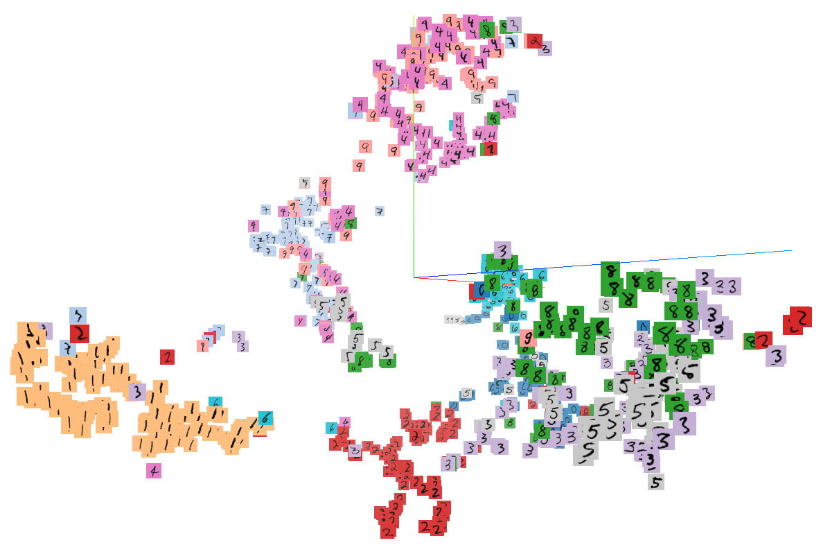
There are some clusters that are relatively homogeneous, like the left one, which is predominantly composed of 1s, or the red cluster composed of 2s. On the other hand, the low-dimensional embedding struggles to distinguish between 5s and 3s. If we wanted to classify images, the low-dimensional representation would likely not yield great results. Of course, one could make the autoencoder deeper or increase the size of the low-dimensional embedding, which I encourage you to explore.

Convolutions and data format

If you are running the code on a GPU, there is a technical detail related to how convolutions are implemented and how images are represented in memory. In the code above, I assumed that the last dimension corresponds to the color channel, which is of size 1 for the input and corresponds to the number of feature maps otherwise. Thus, convolutions would operate on 4D Tensors of size $\text{batch size} \times \text{height} \times \text{width} \times \text{channels}$. This is TensorFlow’s default format. Unfortunately, NVIDIA’s cuDNN routines are optimized for a different data format, where the channel dimension comes before the spatial dimensions, i.e., tensors are of the format $\text{batch size} \times \text{channels} \times \text{height} \times \text{width}$. After reordering dimensions, you have to call tf.contrib.layers.conv2d with the argument data_format="NCHW", instead of the default data_format="NHWC". The speed-up can be substantial, on a p2xlarge AWS instance, this increased the training speed from 27 iterations per second to 40 iterations per second. In my code, you just have to change this line to use the alternative data format.

I hope my code provides a starting point for convolutional autoencoders in TensorFlow. If you want to learn more about convolutional neural networks, check out the links at the bottom.

References

• Recent Advances in Convolutional Neural Networks
• Technical report on convolution arithmetic
• An Introduction to different Types of Convolutions in Deep Learning