Denoising Autoencoder as TensorFlow estimator

Dec 22, 2017 9 min read

I recently started to use Google’s deep learning framework TensorFlow. Since version 1.3, TensorFlow includes a high-level interface inspired by scikit-learn. Unfortunately, as of version 1.4, only 3 different classification and 3 different regression models implementing the Estimator interface are included. To better understand the Estimator interface, Dataset API, and components in tf-slim, I started to implement a simple Autoencoder and applied it to the well-known MNIST dataset of handwritten digits. This post is about my journey and is split in the following sections:

I will assume that you are familiar with TensorFlow basics. The full code is available at https://github.com/sebp/tf_autoencoder. A second part on Convolutional Autoencoders is available too.

Estimators

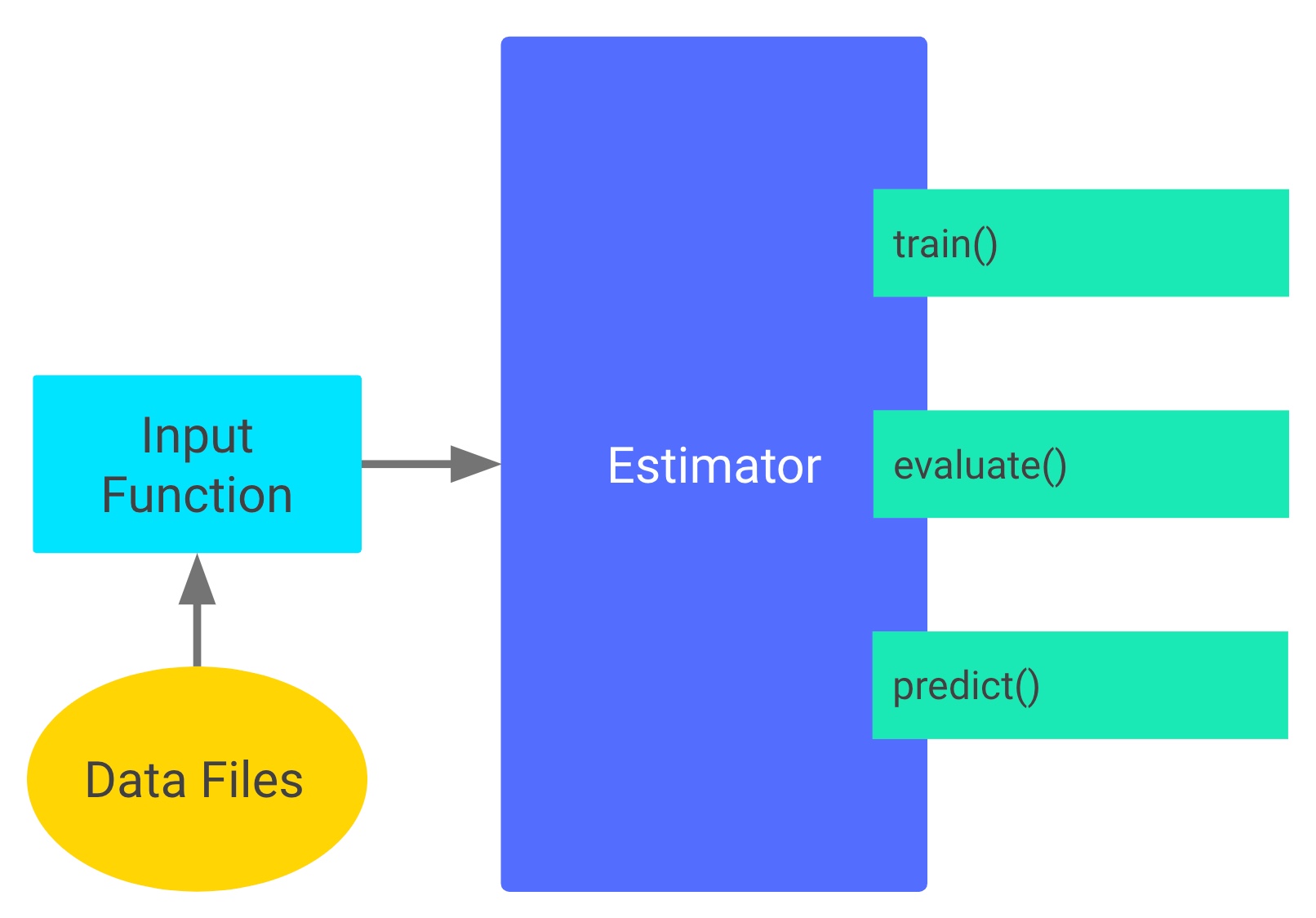
The tf.estimator.Estimator is at the heart TenorFlow’s high-level interface and is similar to Kera’s Model API. It hides most of the boilerplate required to train a model: managing Sessions, writing summary statistics for TensorBoard, or saving and loading checkpoints. An Estimator has three main methods: train, evaluate, and predict. Each of these methods requires a callable input function as first argument that feeds the data to the estimator (more on that later).

Custom estimators

You can write your own custom model implementing the Estimator interface by passing a function returning an instance of tf.estimator.EstimatorSpec as first argument to tf.estimator.Estimator.

def model_fn(features, labels, mode):
    …
    return tf.estimator.EstimatorSpec(
        mode=mode,
        predictions=predictions,
        loss=total_loss,
        train_op=train_op,
        eval_metric_ops=eval_metric_ops)

The first argument – mode – is one of tf.estimator.ModeKeys.TRAIN, tf.estimator.ModeKeys.EVAL or tf.estimator.ModeKeys.PREDICT and determines which of the remaining values must be provided. In TRAIN mode:

loss: A Tensor containing a scalar loss value.
train_op: An Op that runs one step of training. We can use the return value of tf.contrib.layers.optimize_loss here.

In EVAL mode:

loss: A scalar Tensor containing the loss on the validation data.
eval_metric_ops: A dictionary that maps metric names to Tensors of metrics to calculate, typically, one of the tf.metrics functions.

In PREDICT mode:

predictions: A dictionary that maps key names of your choice to Tensors containing the predictions from the model.

An important difference to the Estimators included with TensorFlow is that we need to call relevant tf.summary functions in model_fn ourselves. However, the Estimator will take care of writing summaries to disk so we can inspect them in TenorBoard.

Autoencoder model

The Autoencoder model is straightforward, it consists of two major parts: an encoder and an decoder. The encoder has an input layer (28*28 = 784 dimensions in the case of MNIST) and one or more hidden layers, decreasing in size. In the decoder, we reverse the operations of the encoder by blowing the output of the smallest hidden layer up to the size of the input (optionally, with hidden layers of increasing size in-between). The loss function computes the difference between the original image and the reconstructed image (the output of the decoder). Common loss functions are mean squared error and cross-entropy.

To construct the encoder network, we specify a list containing the number of hidden units for each layer and (optionally) add dropout layers in-between:

def encoder(inputs, hidden_units, dropout, is_training):
    net = inputs
    for num_hidden_units in hidden_units:
        net = tf.contrib.layers.fully_connected(
            net, num_outputs=num_hidden_units)
        if dropout is not None:
            net = slim.dropout(net, is_training=is_training)
        add_hidden_layer_summary(net)
    return net

where add_hidden_layer_summary adds a histogram of the activations and the fraction of non-zero activations to be displayed in TensorBoard. The latter is particularly useful when debugging networks with rectified linear units (ReLU). If too many hidden units return 0 values early during optimization, the model won’t be able to learn anymore, in which case one would typically try to lower the learning rate or choose a different activation function. The network of the decoder is almost identical, we just explicitly use a linear activation function (activation_fn=None) and no dropout in the last layer:

def decoder(inputs, hidden_units, dropout, is_training):
    net = inputs
    for num_hidden_units in hidden_units[:-1]:
        net = tf.contrib.layers.fully_connected(
            net, num_outputs=num_hidden_units)
        if dropout is not None:
            net = slim.dropout(net, is_training=is_training)
        add_hidden_layer_summary(net)

    net = tf.contrib.layers.fully_connected(net, hidden_units[-1],
                                            activation_fn=None)
    tf.summary.histogram('activation', net)
    return net

You may have noticed that we did no specify any activation function so far. Thanks to TenorFlow’s arg_scope context manager, we can easily set the activation function for all fully connected layers. At the same time we set an appropriate weight initializer and (optionally) use weight decay:

def autoencoder(inputs, hidden_units, activation_fn, dropout, weight_decay, mode):
    is_training = mode == tf.estimator.ModeKeys.TRAIN

    weights_init = slim.initializers.variance_scaling_initializer()
    if weight_decay is None:
        weights_regularizer = None
    else:
        weights_reg = tf.contrib.layers.l2_regularizer(weight_decay)

    with slim.arg_scope([tf.contrib.layers.fully_connected],
                        weights_initializer=weights_init,
                        weights_regularizer=weights_reg,
                        activation_fn=activation_fn):
        net = encoder(inputs, hidden_units, dropout, is_training)
        n_features = inputs.shape[1].value
        decoder_units = hidden_units[:-1][::-1] + [n_features]
        net = decoder(net, decoder_units, dropout, is_training)
    return net

where slim.initializers.variance_scaling_initializer corresponds to the initialization of He et al., which is the current recommendation for networks with ReLU activations. This concludes the architecture of the autoencoder. Next, we need to implement the model_fn function passed to tf.estimator.Estimator as outlined above.

Autoencoder model_fn

First, we construct the network’s architecture using the autoencoder function described above:

logits = autoencoder(inputs=features,
                     hidden_units=hidden_units,
                     activation_fn=activation_fn,
                     dropout=dropout,
                     weight_decay=weight_decay,
                     mode=mode)

Subsequent steps depend on the value of mode. In prediction mode, we merely have to return the reconstructed image, therefore we make sure all values are within the interval [0; 1] by applying the sigmoid function:

probs = tf.nn.sigmoid(logits)
predictions = {"prediction": probs}
if mode == tf.estimator.ModeKeys.PREDICT:
    return tf.estimator.EstimatorSpec(
        mode=mode,
        predictions=predictions)

In training and evaluation mode, we need to compute the loss, which is cross-entropy in this example:

tf.losses.sigmoid_cross_entropy(labels, logits)
total_loss = tf.losses.get_total_loss(add_regularization_losses=is_training)

The second line is needed to add the $\ell_2$-losses used in weight decay. Most importantly, training relies on choosing an optimizer, here we use Adam and an exponential learning rate decay. The latter dynamically updates the learning rate during training according to the formula $$ \text{decayed learning rate} = \text{base learning rate} \cdot 0.96^{\lfloor i / 1000 \rfloor} , $$ where $i$ is the current iteration. It would probably work as well without learning rate decay, but I included it for the sake of completeness.

if mode == tf.estimator.ModeKeys.TRAIN:
    train_op = tf.contrib.layers.optimize_loss(
        loss=total_loss,
        optimizer="Adam",
        learning_rate=learning_rate,
        learning_rate_decay_fn=lambda lr, gs: tf.train.exponential_decay(lr, gs, 1000, 0.96, staircase=True),
        global_step=tf.train.get_global_step(),
        summaries=["learning_rate", "global_gradient_norm"])

    # Add histograms for trainable variables
    for var in tf.trainable_variables():
        tf.summary.histogram(var.op.name, var)

Note that we add a histogram of all trainable variables for TensorBoard in the last part.

Finally, we compute the root mean squared error when in evaluation mode:

if mode == tf.estimator.ModeKeys.EVAL:
    eval_metric_ops = {
        "rmse": tf.metrics.root_mean_squared_error(
            tf.cast(labels, tf.float64), tf.cast(probs, tf.float64))
    }

and return the specification of our autoencoder estimator:

return tf.estimator.EstimatorSpec(
    mode=mode,
    predictions=predictions,
    loss=total_loss,
    train_op=train_op,
    eval_metric_ops=eval_metric_ops)

Feeding data to an Estimator via the Dataset API

Once we constructed our estimator, e.g. via

estimator = AutoEncoder(hidden_units=[128, 64, 32],
                        dropout=None,
                        weight_decay=1e-5,
                        learning_rate=0.001)

we would like to train it by calling train, which expects a callable that returns two tensors, one representing the input data and one the groundtruth data. The easiest way would be to use tf.estimator.inputs.numpy_input_fn, but instead I want to introduce TensorFlow’s Dataset API, which is more generic.

The Dataset API comprises two elements:

tf.data.Dataset represents a dataset and any transformations applied to it.
tf.data.Iterator is used to extract elements from a Dataset. In particular, Iterator.get_next() returns the next element of a Dataset and typically is what is fed to an estimator.

Here, I’m using what is called an initializable Iterator, inspired by this post. We define one placeholder for the input image and one for the groundtruth image and initialize the placeholders before training starts using a hook. First, let’s create a Dataset from the placeholders:

placeholders = [
    tf.placeholder(data.dtype, data.shape, name='input_image'),
    tf.placeholder(data.dtype, data.shape, name='groundtruth_image')
]
dataset = tf.data.Dataset.from_tensor_slices(placeholders)

Next, we shuffle the dataset and allow retrieving data from it until the specified number of epochs has been reached:

dataset = dataset.shuffle(buffer_size=10000)
dataset = dataset.repeat(num_epochs)

When creating input for evaluation or prediction, we are going to skip these two steps.

Finally, we combine multiple elements into a batch and create an iterator from the dataset:

dataset = dataset.batch(batch_size)

iterator = dataset.make_initializable_iterator()
next_example, next_label = iterator.get_next()

To initialize the placeholders, we need to call tf.Sesssion.run with

feed_dict = {placeholders[0]: input_data, placeholders[1]: groundtruth_data}

Since the Estimator will create a Session for us, we need a way to call our initialization code after the session has been created and before training begins. The Estimator’s train, evaluate and predict methods accept a list of SessionRunHook subclasses as the hooks argument, which we can use to inject our code in the right place. Therefore, we first create a generic hook that runs after the session has been created:

class IteratorInitializerHook(tf.train.SessionRunHook):
    """Hook to initialise data iterator after Session is created."""

    def __init__(self):
        self.iterator_initializer_func = None

    def after_create_session(self, session, coord):
        """Initialise the iterator after the session has been created."""
        assert callable(self.iterator_initializer_func)
        self.iterator_initializer_func(session)

To make things a little bit nicer, we create an InputFunction class which implements the __call__ method. Thus, it will behave like a function and we can pass it directly to tf.estimator.Estimator.train and related methods.

class InputFunction:
    def __init__(self, data, batch_size, num_epochs, mode):
        self.data = data
        self.batch_size = batch_size
        self.mode = mode
        self.num_epochs = num_epochs
        self.init_hook = IteratorInitializerHook()

     def __call__(self):
        # Define placeholders
        placeholders = [
            tf.placeholder(self.data.dtype, self.data.shape, name='input_image'),
            tf.placeholder(self.data.dtype, self.data.shape, name='reconstruct_image')
        ]

        # Build dataset pipeline
        dataset = tf.data.Dataset.from_tensor_slices(placeholders)
        if self.mode == tf.estimator.ModeKeys.TRAIN:
            dataset = dataset.shuffle(buffer_size=10000)
            dataset = dataset.repeat(self.num_epochs)
        dataset = dataset.batch(self.batch_size)

        # create iterator from dataset
        iterator = dataset.make_initializable_iterator()
        next_example, next_label = iterator.get_next()

        # create initialization hook
        def _init(sess):
            feed_dict = dict(zip(placeholders, [self.data, self.data])
            sess.run(iterator.initializer,
                     feed_dict=feed_dict)

        self.init_hook.iterator_initializer_func = _init

        return next_example, next_label

Finally, we can use the InputFunction class to train our autoencoder for 30 epochs:

from tensorflow.examples.tutorials.mnist import input_data as mnist_data

mnist = mnist_data.read_data_sets('mnist_data', one_hot=False)
train_input_fn = InputFunction(
    data=mnist.train.images,
    batch_size=256,
    num_epochs=30,
    mode=tf.estimator.ModeKeys.TRAIN)
autoencoder.train(train_input_fn, hooks=[train_input_fn.init_hook])

The video below shows ten reconstructed images from the test data and their corresponding groundtruth after each epoch of training:

Denoising Autoencoder

A denoising autoencoder is slight variation on the autoencoder described above. The only difference is that input images are randomly corrupted before they are fed to the autoencoder (we still use the original, uncorrupted image to compute the loss). This acts as a form of regularization to avoid overfitting.

noise_factor = 0.5  # a float in [0; 1)

def add_noise(input_img, groundtruth_img):
    noise = noise_factor * tf.random_normal(input_img.shape.as_list())
    input_corrupted = tf.clip_by_value(tf.add(input_img, noise), 0., 1.)
    return input_corrupted, groundtruth

The function above takes two Tensors representing the input and groundtruth image, respectively, and corrupts the input image by the specified amount of noise. We can use this function to transform all of the images using Dataset’s map function:

dataset = dataset.map(add_noise, num_parallel_calls=4)
dataset = dataset.prefetch(512)

The function passed to map will be part of the compute graph, thus you have to use TensorFlow operations to modify your input or use tf.py_func. The num_parallel_calls arguments speeds up preprocessing significantly, because multiple images are transformed in parallel. The second line ensures a certain amount of corrupted images are precomputed, otherwise the transformation would only be applied when executing iterator.get_next(), which would result in a delay for each batch and bad GPU utilization. The video below shows the groundtruth, input and output of the denoising autoencoder for up to 60 epochs: